Chris Meyer, Past President, Ontario Association of Physics Teachers
chris_meyer1@sympatico.ca

At times electrons can seem awfully clever, as if they talk to one another and plan what each will do: “okay, so you two go along that path and I'll go along this one” or “I'll only give up ¼ of my energy here because the next load has a higher resistance and I need to give it ¾ of my energy”. How do they pull off these amazing feats of collaboration and foresight? For years I was genuinely stumped when trying to explain the rationale behind series and parallel phenomena; my attempts were all variations of “well, because that’s what happens”.

How do electrons “know” that there is another resistor connected in series down the road? How do they “know” which parallel path to choose? For that matter, how does a battery connected to a single resistor “know” how much current to push? There are so many mysteries of simple electric circuits! Let's explore the last question first, which will help us answer all the others.

To know or not to know, that is the question
First of all, using the verb “to know” in these situations is a quaintly inappropriate anthropomorphization of electrons: after all, they don't “know” anything! Instead, let’s adjust our vocabulary to ask a scientific question: how does a battery connected to a single resistor establish a steady state of current that accounts for the resistance of the circuit? It’s easy to see why the anthropomorphic language is so appealing: it’s much simpler! I will continue with some colloquial language in this article since this is what is heard in the classroom, but I will always provide a translation into proper scientific jargon.

How deep should we dive into DC circuits?
There are many levels at which we can explain the workings of a DC circuit. The simplest level describes the patterns of its macroscopic characteristics: current, voltage, and resistance. This is the level of most high school or introductory university instruction and is a level that is pedagogically quite reasonable. However, this level doesn't provide a microscopic physical model that answers the common questions of “how?” or “why?” and this bugs some people an awful lot (hopefully this you; read on!). In this article, I offer two levels of explanation that run “parallel” with one another: the main narrative, and “deeper dive” segments that provide background information and more detailed explanations. I encourage you to dive deep!

What a battery really, really wants
So, what does a battery really want to do? Translation: what is the function of a source in a circuit? Simply put, to move electrons from one side of it to the other, adding energy to the system of electrons. In the absence of much resistance to the movement of these electrons, most sources have the ability to drive very large currents, at least for a while, like during a short circuit. In this article, we won’t focus on the internal workings of the source, which might consist of chemical reactions in a battery or of movement and force in a Van de Graaff generator.

Deeper dive: conduction electrons. The electrons that form a current are mobile, meaning they are not bound to a particular atom and can easily move through the crystal lattice of a solid metal in response to external electric fields. We call these the conduction electrons. (Even deeper: the wave function of a conduction electron is spread fairly evenly throughout the metal rather than being localized near a few atoms like in a molecular orbital.)

Deeper dive: conduction electrons don’t push each other along. As metal atoms bond to form a crystal lattice (a solid piece of metal), for every conduction electron that is freed up from an atom, there is a positively charged ionic core that is left behind. Taken together, the conduction electrons and ionic cores produce a net electric field of zero. As a result, conduction electrons don’t interact electrically with one another: for every neighboring conduction electron that might repel, there is a positively charged ion attracting, yielding a net force of zero. So, conduction electrons don’t “push each other around” or repel each other inside a metal. Instead, an external electric field from a source outside the system of conduction electrons must do the pushing.

The electron pileup
Before we consider how a source behaves in a circuit, let’s consider a source in isolation. An active source will do its job for a short duration, even while disconnected from a circuit! This results in extra electrons piling up at one end of the source and a deficit of electrons at the other. After a very short while, additional electrons will stop arriving at the negative terminal: any newcomer electrons are repelled by the pileup. The opposite happens at the positive terminal where the net positive charge becomes so great that the source can no longer remove electrons from that region. The electrons in the source soon arrive at a state of static equilibrium, unable to move until the equilibrium is disturbed. This excess and deficit of electrons is very hard to detect on a AA battery (you don’t get shocked from touching a terminal) but is quite evident and entertaining on a Van de Graaff generator! The piling up of electrons functions as a feedback mechanism that regulates or moderates the electrons’ behaviour: this is the key idea we will use to explain all the mysteries of direct current electric circuits.

Deeper dive: drift speed. When an external electric field drives a current in a wire, the conduction electrons regularly bump into the atoms of the metal, which slows them down greatly. If you average out all the bumping, you get an overall speed for the conduction electrons that is called their drift speed. This is the speed of the current in most circuits and is very slow, typically fractions of a millimeter per second! We can liken this to flowing water, which has a slow speed associated with its bulk (like a river current) and a very fast speed from the random thermal vibrations of individual water molecules that are bumping into one another.

Deeper dive: sea of electrons. It is helpful to think of the collection of conduction electrons as a sea of electrons, where we ignore the random motion of individual electrons and focus on the movement of the group. This helps us better understand pileups, which form on a timescale of billionths of a second. Since pileups happen in such little time, it is tempting to think that electrons are moving quickly, but this is not the case owing to their leisurely drift speed! Since there are so many conduction electrons (in a copper wire there are roughly 1.3 conduction electrons per copper atom), it takes very little time for an external field to move the sea of electrons a very short distance and create a large pileup.

Deeper dive: surface charge. The sea of electrons is regularly driven into the surface of a metal or to its interface with another material. This causes electrons to be pushed up onto the surface of the metal where they outnumber the positively charged ionic cores; this is the start of a pileup. Electrons will continue to accumulate on the surface until the surface electrons produce a large enough electric field of their own to balance the field driving the conduction electrons to the surface; this is the finish of the pileup’s formation. A better name for a “pileup” is “surface charge”: a region of non-zero net charge on the surface of a metal (a positive surface charge can occur if the sea of electrons is driven away from the surface). How do the surface charges in a circuit compare with those of a charged or polarized metal object? On the one hand, very similar: they are regions of non-zero net charge. On the other hand, different: the surface charges in a circuit are not static (i.e., membership in the pileup is always changing) and their size can be very small (one or two surface electrons can cause current to turn a corner in a circuit).


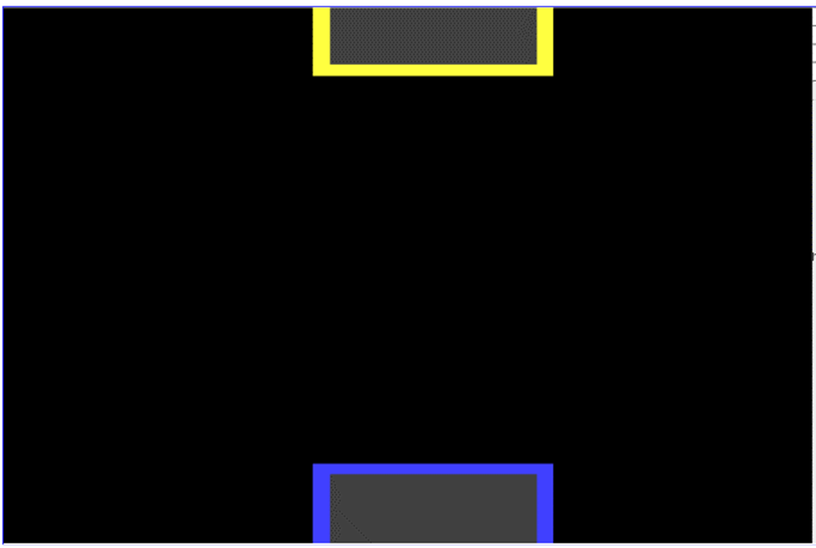Figure 1: A simulation showing the oppositely charged terminals of the source.

To help picture the pileups of electrons, consider figure 1 showing two oppositely charged blocks of metal that I set up in a simulation (information on the simulation is at the end of the article). The gray region represents metal and the colours represent regions of non-zero net charge. I will choose yellow to be a negative net charge (the pileup of electrons) and blue positive (the deficit). Together these two charged blocks represent the oppositely charged terminals of the source. At the moment, these charges are static, since there is no circuit allowing them to move. Notice that the net charge is only found on the surface of the metal. All the pileups we discuss are surface charges and are found on the surface of the conductors, never in the interior, as described in the deeper dives.

How does the source know?
Time to consider a simple circuit: a source, two wires, and a resistor. We are now ready to answer one of our questions: how does the source know how much current to push? Translation: How does it create a steady state current that accounts for the resistance of the circuit? Once we connect the two wires to the source, the electrons piled up at the negative terminal see open waters! A ripple of electrons, like a wave, rushes along the wire’s surface and soon piles up at the boundary of the wire and resistor. The “height” of this pileup (the charge density) depends on both the amount of resistance provided by the resistor and the strength of the source. And in extent, the pileup goes all the way back to the source! This is how a source “knows” there is a resistor further down the wire. Electrons in the wire feel a combination of two effects: a forward force due to the pileup on the source and a backward force due to the pileup at the resistor. The result is a small net force forwards, as opposed to a short circuit with a large net force forwards, resulting in an electron current moderated by the circuit’s resistance. The opposite happens starting at the other terminal of the battery, with a deficit of electrons taking the role of the pileup. There is a lot of interesting detail and subtlety that this explanation glosses over! Figure 2 shows our simple circuit in the simulator:


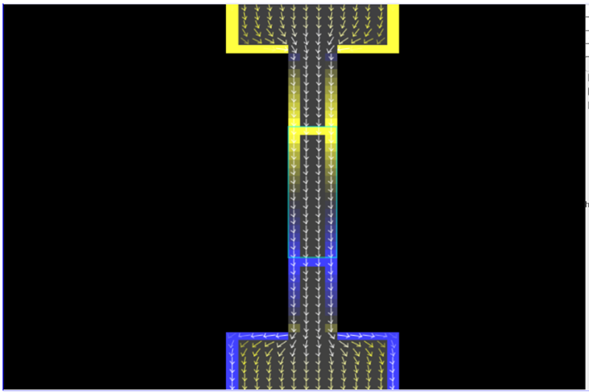Figure 2: A resistor connected by two wires to the oppositely charged terminals of a source.

While the simple circuit is operating, the source works hard to maintain a pileup of electrons at its negative terminal. Notice the pileup at the negative side of the resistor (a yellow horizontal bar in the simulation above). Its “height” is a bit smaller than that of the source, leading to a small voltage drop across the wire (a realistic wire always has a small resistance). So, the difference in “height” of adjacent pileups is related to the voltage drop: a greater difference in pileup heights produces a larger forwards force, more work is done, more energy is transferred, producing a larger voltage drop. At the far end of the resistor is a deficit of electrons (the opposite of a pileup, the blue horizontal bar). This makes for a large difference in pileup heights across the resistor: notice the large change in colours from bright yellow to blue. In fact, the drop across the resistor is almost the same size as the original voltage drop between the source terminals, the difference coming from the very small drops in the two wires.

Deeper dive: rapidly adjusting surface charge. When the wires are connected, conduction electrons are driven away from the negative terminal of the source at a rate greater than the resistor can handle. This leads to a growing accumulation of electrons on the surface of the wire at the boundary with the resistor, causing two things to happen: an increasing amount of current starts to be driven through the resistor and a decreasing amount of current gets driven from the source to the resistor. On a timescale of nanoseconds, the current from the source reduces enough to match the growing current through the resistor. The surface charges now stabilize and the circuit reaches the steady state of current flow that we talk about in our classes, all before any electron is able to move more than an atomic diameter! The wave-like effect of shifting charge rippling along the surface quickly creates a surface charge distribution that allows the source and distant resistor to affect one another. This is why a flick of a switch will turn on a light almost instantly, even though it would take electrons many minutes to move the distance from a switch to a light in the DC circuits we build.

Deeper, deeper dive: things get polarized. Even before the source is connected to the wires, the electric field due to the charge build up on the source polarizes the wires and resistor. This means there are already pileups in the wires before they are connected! This doesn't change the basic process of a rapidly adjusting surface charge, but it does change the details before the steady state is arrived at.


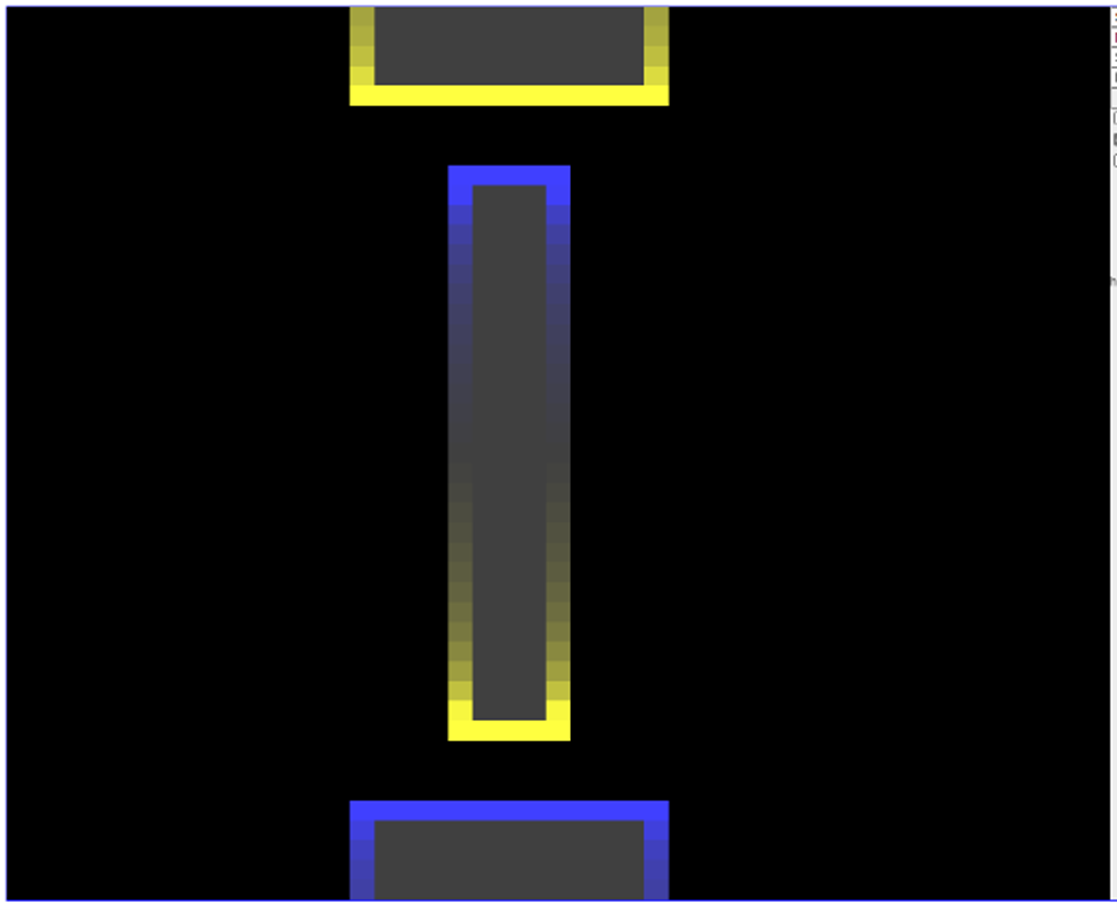
Figure 3: The wires and resistor of the simple circuit are polarized just before connecting with the source terminals.

Deeper dive: the surface charge gradient drives current. Once the circuit has settled down, there is now a gradient of surface charge along the length of the wire or resistor that creates a constant electric field in the forward direction inside the wire to drive the conduction electrons. The larger the gradient, the larger the electric field and electron current. No gradient, no current. Based on this understanding, we can associate the gradient of the surface charge with the voltage drop. You may have learned that electric fields inside a conductor are zero, but this is only the case in static situations. Electric circuits involve moving charges; this requires a steady force to drive current against resistance, which means there must be a non-zero electric field inside the wire, in this case produced by the gradient of surface charge.


This video shows evidence for the existence of the surface charge gradient that drives the current in a wire. A very large voltage is required to create a noticeable surface charge.

Deeper dive: the job of a source. Conduction electrons are driven primarily by the field due to surface charge along wires or resistors, so they are not directly driven by the source. Energy transfers from the field of the surface charges to the conduction electrons. So, what is the role of the source? It must provide the energy to create and maintain the surface charge, whose electrons are not static and need to be constantly replaced. This requires the continuous operation of the source to move electrons and transfer energy to the surface of the circuit. Turn off the source, surface charges dissipate (pileups combine with deficits), and currents stop.

Energy in a simple circuit
When I discuss energy in a circuit with my grade nine students, we start by defining the system of conduction electrons. A source adds energy to the system of electrons and a load removes energy from it; energy transfers in and out of the system due to interactions in the source and the load. Here is an energy flow diagram for this grade 9 explanation:


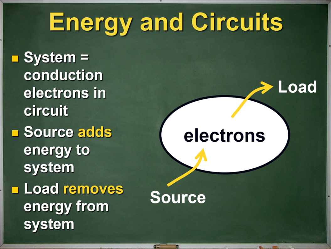Figure 4: An energy flow diagram for a simple circuit from my grade nine science class.

Let’s refine this picture to reflect three new ideas from our discussions here: the source expends its energy creating the pileups (the surface charge), the pileups drive the conduction electrons (the current), and the conduction electrons transfer their energy to the atoms of the load or wire through collisions. We will also include labels describing how the energy is stored. An improved energy flow diagram looks like this:


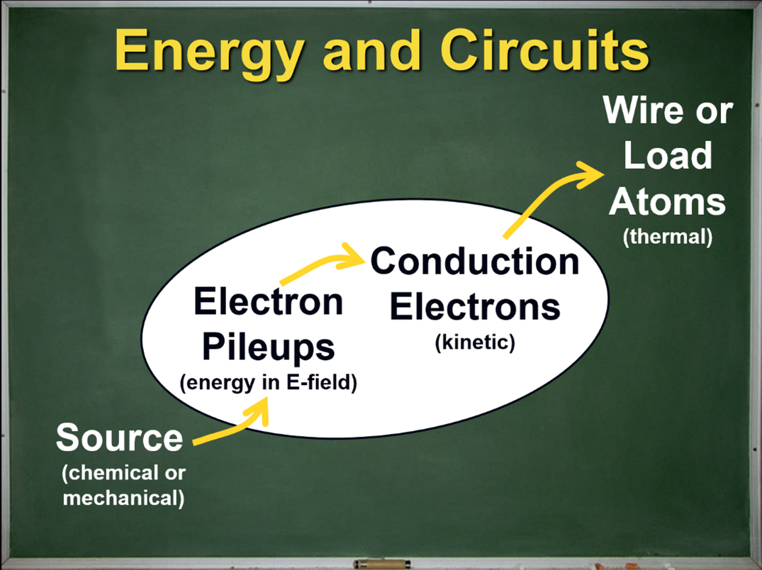Figure 5: An improved energy flow diagram that distinguishes between conduction electrons and surface charge electrons (pileups).

Which way? The puzzle of parallel connections
So, it’s all about pileups! Now I think you are ready to try your own explanation for how electrons “know” which path of a parallel circuit to take. Suppose we add a second path to our previous simple circuit that includes a smaller resistor. Take a moment right now before you read on: use the idea of pileups or surface charge to explain the puzzle of parallel circuits.

We must solve this conundrum: how do electrons at a junction point “know” that one path has more resistance than another when those resistors are far down the wires? Pileups! When the wires are first connected to the source, a ripple of electrons rushes equally along each path of the circuit, initially oblivious to the existence of the distant resistors. When the ripples reach the resistors, new pileups form with sizes related to the amount of resistance along that path (which is different) and the strength of the source (which is the same). The pileups extend back along the surface of the branches of the circuit to the junction point. Electrons at the junction point will feel a smaller push forward along the high resistance path and a larger push forward along the low resistance path. So, no need for the electrons to “know” anything, they just respond to the forces present near the junction point. The pileup effect continues past the junction and all the way back to the source, providing feedback that adjusts how much current the source drives into the circuit. In this case, less feedback leads to more current through the source terminals.

Deeper dive: surface charge feedback. Suppose electrons at the junction point in our parallel circuit became “confused” or for some reason more electrons travel down the high resistance path than ought to (perhaps due to some randomness on a microscopic level). This would cause the surface charge along that path to become just slightly larger and decrease the electric field parallel to that path, causing less current to be driven along it. The slight excess of current leads to a feedback effect that brings the current back down to the normal, steady state value. The feedback between current and surface charge is what ensures the consistent macroscopic patterns of current that we are familiar with.

Let’s take a look at the parallel example using the simulation. Unfortunately, the simulation I use does not show the ripples and changing pileups in action; it only shows the steady state result. So instead, I will show steps with small, incremental changes to the construction of the circuit.


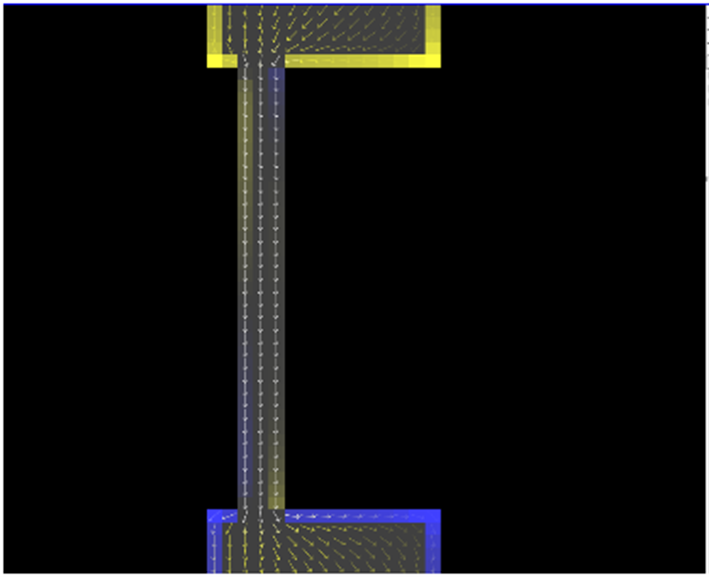Figure 6: The first step in building a parallel circuit. A single wire (without a resistor) is connected between the two source terminals.


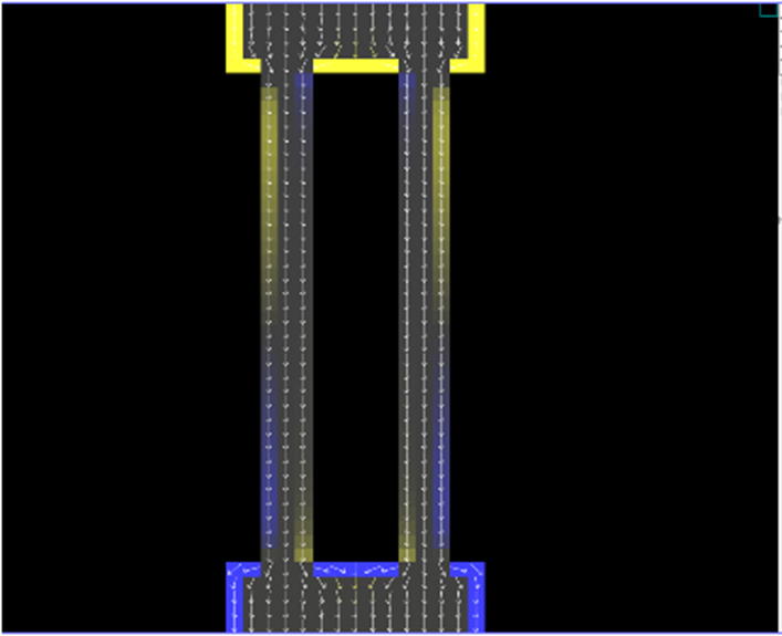Figure 7: A second wire (again without a resistor) is connected between the two source terminals.

In the two images above, we see the terminals of the source, the negative (yellow) at the top and the positive (blue) at the bottom. In figure 6, a thin wire with some resistance connects the two terminals, allowing current to flow that is represented by the small arrows of varying intensity: white indicates large current, fading yellow represents small current. Figure 7 shows a second thin wire connecting the terminals of the source. Looking carefully at the arrows, we can see more bright white arrows in the terminals indicating more current flowing overall.


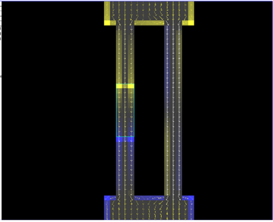Figure 8: A weak resistor is added to the first path of the circuit.

Figure 8 shows a resistor added into the first wire. There is a pileup of electrons (the yellow horizontal bar) at the negative side of the resistor. We can also see how the pileup extends back toward the source. There is a deficit of electrons (the blue horizontal bar) on the positive side of the resistor. The yellow arrows indicate less current traveling along this path compared to the other (white arrows).


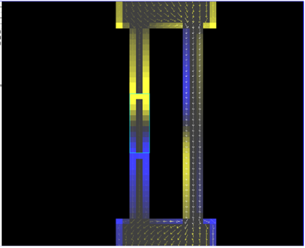Figure 9: The strength of the first resistor is increased.

In figure 9, the resistance along the first path is greatly increased causing the size of the pileups to increase. Now almost all the voltage drop occurs within the resistor rather than along the length of the wire (the resistor goes from bright yellow to bright blue, a large pileup to a large deficit). Now there is very little current traveling through this wire, indicated by the dim arrows. The pileups are having a strong effect all the way back to the terminals of the source.


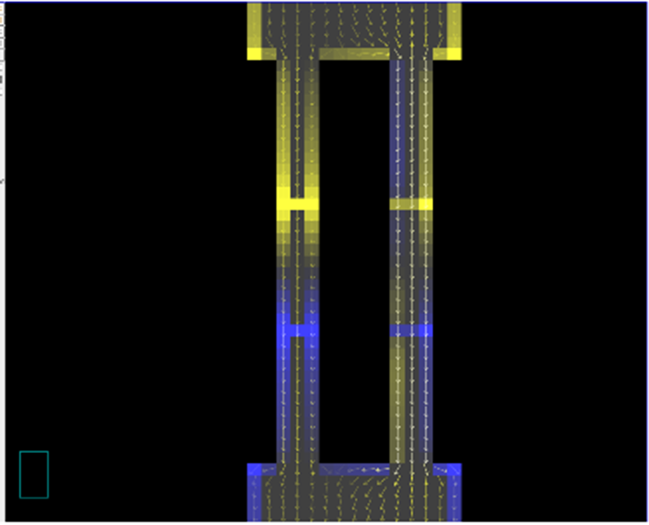Figure 10: A second smaller resistor is added along the second path of the circuit.

Finally, we add a smaller resistor to the second wire. The simulation shows a smaller pileup and larger current along this path. We have now completed our two-resistor parallel circuit. The two resistors have pileups of different heights that extend back to the junction and cause different amounts of current to flow along each path.

How much? The puzzle of series connections
The last puzzle for us to solve is that of voltages in a series connection. Let's explore what happens when current travels through a small and then large resistor. How do the electrons “know” that they should only give up a small part of their energy in the first resistor and the rest in the second? (Translation: Why is there a small transfer of energy to the first resistor and a large transfer to the second?) I encourage you to try making your own explanation, following the reasoning we presented in the discussion of the simple circuit. Hint: use the reasoning twice, but with a bonus that connects what happens at each resistor!

Let’s tell the story of this series circuit by tracing the sequence of pileups that occur. Recall that we initially had a pileup of electrons on the negative terminal of the source before it was connected to the circuit. After connecting, a ripple of electrons travels along the wire and reaches the boundary to the first resistor. Here a new pileup forms that slows the incoming current. Since the first resistor has a small resistance, the pileup is small and a fairly large current passes through it (white arrows), oblivious for the moment to the second resistor:


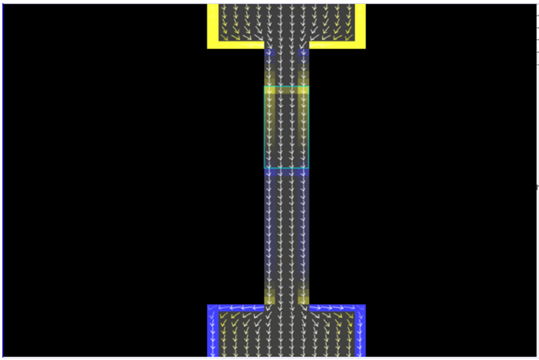Figure 11: The electron current reaches the first of two resistors connected in series.

Notice that the pileup on the negative side of the resistor is small (the colours are faint), which means that a large current will flow through it. The gradient of colour along this resistor is not especially large (going only from a medium yellow to a neutral grey). The wire before and after this resistor has a resistance and so it is noticeably taking some of the voltage drop from source.
The ripple continues out of the first resistor, along a middle wire, and reaches the boundary of the second resistor. Here the resistance is much greater, so a second larger pileup forms, which slows down the current even more. But wait! This large slowdown causes the second pileup to extend back through the first resistor and all the way to the source! Now the first resistor has a smaller difference in pileups across its length; its voltage drop reduces!


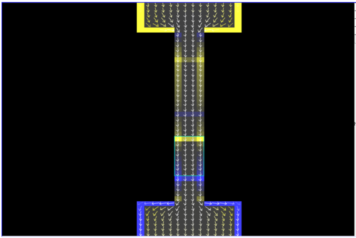Figure 12: The current reaches the second of two resistors connected in series.

In figure 12 we see the colours in the first resistor only change from a medium yellow to a dim yellow, representing a smaller voltage drop. Meanwhile, the larger pileup in front of the second resistor produces a larger colour change across it (brighter yellow to bright blue), indicating a large voltage drop. There is a bit of rippling back and forth while the pileups sort themselves out. But soon, in less than a billionth of a second, the ripples settle down, leaving a steady state of current that we recognize from our teaching: the current is the same everywhere along this single path and is at a lower value than with the single resistor; also, the total voltage rise equals the total voltage drop where the drop of the first resistor is smaller than the drop of the second. And it was all sorted out through pileups!

Should we share these secrets?
I remember in my second year E&M class, my professor (the awesome John Pitre, a storied OAPT member) casually mentioned that all this circuit stuff could be explained by “sgfdhj ctsrgh”. I couldn’t quite catch what he said and we didn't return to it anywhere else in our discussions; nor was it in any of my textbooks. So here I am, more than 25 years later finally sorting this out (using my favourite technique for doing this, writing an article!). Should these ideas become a regular part of our introductory lessons on electric circuits? I am not yet sure! I have presented the pileup explanations in a way that could be understandable to grade 11 physics students given a fair bit of time and effort. These explanations might even be useful in grade 9 science for simple off-the-cuff remarks: “oh, electrons just pileup in front of the resistor and slow down the flow of the current,” which is technically correct and conveniently glosses over the complex details of the pileups. I would really like to see a revised grade 12 physics curriculum where we look at surface charge and electric fields inside a circuit; this would form a nice conceptual bridge between grade 9 static electricity, grade 11 circuits, and the grade 12 unit on electric fields (hello, ministry, are you there?). For now, I keep these ideas in my back pocket to share with the handful of students and teachers who ask the question: “How do electrons know what to do?”

Learn more, make your own pileups!
An excellent explanation of surface charge can be found in the textbook of Chabay and Sherwood, who have done the most to work out the pedagogical value of surface charge explanations. In this article, you can track down their references and explore some of the foundational work on this topic, which goes into tremendous detail. Chabay and Sherwood have a fantastic web-based application that visualizes sets of data in three dimensions showing surface charge in very simple circuits. The simulation I used is much simpler. (Brief instructions: make sure you are running the old version of this simulation, select “Setup: wire with resistance”, select “mouse = adds grounded conductor”, clear the screen, and draw your own circuit configurations. Change the mouse so it adjusts conductivity to create resistors or just change the size of your wire! Hours of fun for the whole family!)

Tags: Electricity, Field Theory