Eric Haller, Peel District School Board, Editor of the OAPT Newsletter
eric.haller@peelsb.com

Often, we ask students to do an experiment, gather a set of two-variable data, make a scatter plot, and then try to find the curve of best fit, along with its equation. Historically, Microsoft Excel was the go-to for doing something like this, however nowadays I find my students are most comfortable using Desmos to graph things, because it’s free, simple to use, and doesn’t require any installation or logging in. Desmos is great for making scatter plots and fitting curves, and it can even fit curves beyond Excel’s ‘Add Trendline’ functionality, which is limited to exponential, power, logarithmic, and polynomial-types of curves (Excel can do additional curves, but it's tricky, check out my previous article for instructions on how to do that if you like). In this article, I’d like to go over how you can do a curve of best fit in Desmos, even for complicated curves like what you would find with a damped harmonic oscillator experiment, or with Kepler's third law of planetary motion.

First, let’s quickly go over doing a line of best fit in Desmos. This can be done by adding a table, filling in the x and y-data, and then by typing in a general formula for a line. In Desmos, typing in something like “y=2x+5” will prompt it to graph the function, if instead you want it to do a line of best fit for you, you would type in “y_1~mx_1+b”. The subscripts on the x and y variables indicate to Desmos that you are referring to those specific columns in your data table, and the tilde (~) indicates to Desmos you want it to do a fit of data. Desmos will then try to fit the equation you provided to the points on the graph, giving you the best possible values for the coefficients m and b.


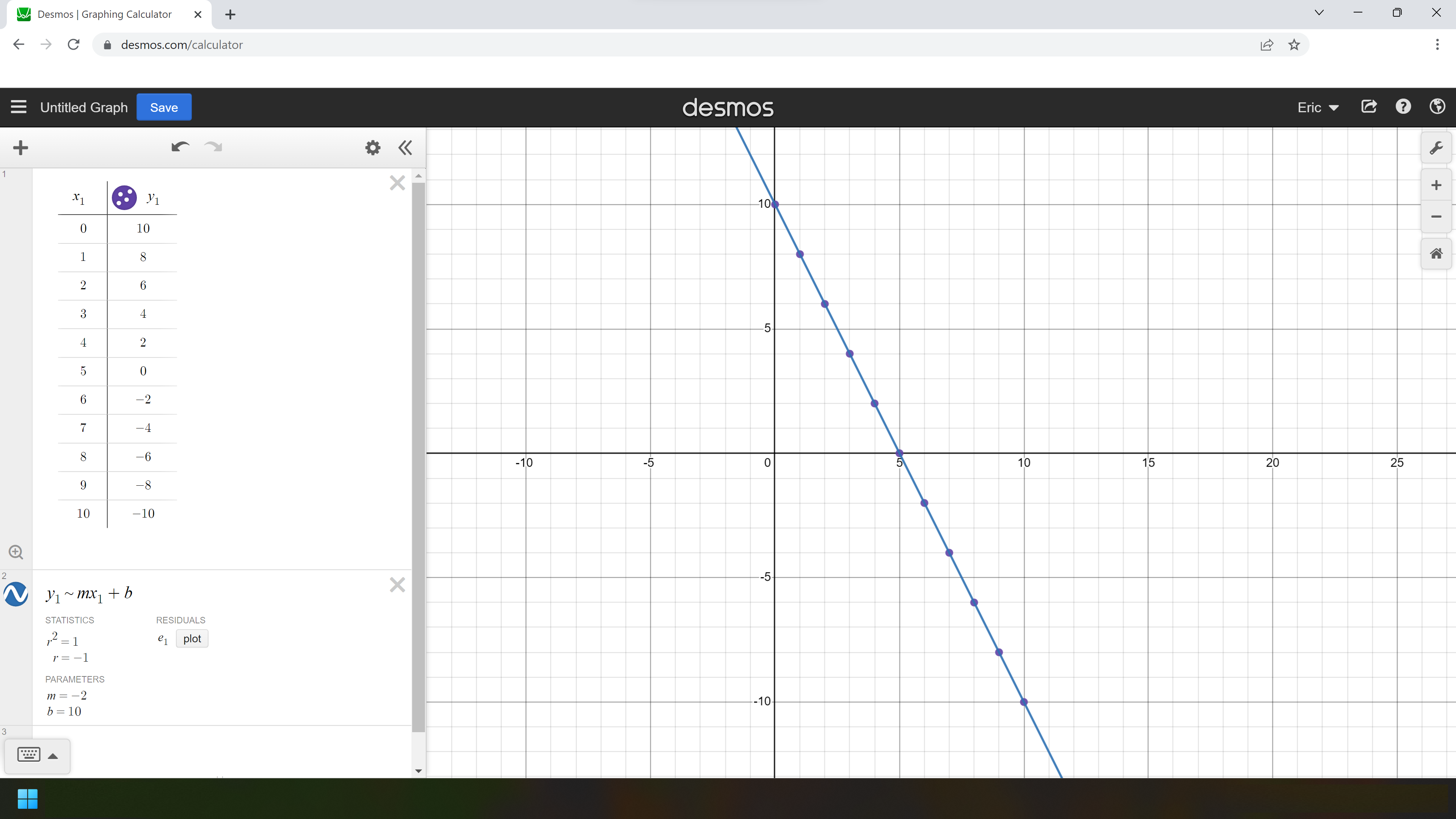Figure 1: A line of best fit done in Desmos, click here to access the file in Desmos.

In the previous example, we asked Desmos to fit a function of the form y = mx + b to the provided data set, and it found m = –2 and b = 10. Thus, the line of best fit would be y = –2x + 10, which it already graphed for comparison.

If we wanted Desmos to fit some other type of curve, we would just have to type in an equation that’s different from “y_1~mx_1+b”. As an example, consider a problem around Kepler's third law of planetary motion, which states that the square of a planet's orbital period is proportional to the cube of the length of the semi-major axis of its orbit. Mathematically, we could write this as a proportionality statement, like T² ∝ r³; or as an equation with a proportionality constant inserted, like T² = kr³. If we had a set of data describing the period and orbital distance for each planet in our solar system, we could use Desmos to find the value of the proportionality constant. Unfortunately, while Desmos can graph implicit plots like y² = kx³, it can’t fit a curve of the form y² = kx³. This isn’t a big issue though, if we square root both sides, it can fit a curve of the form y = sqrt(kx³), and plot the comparison.


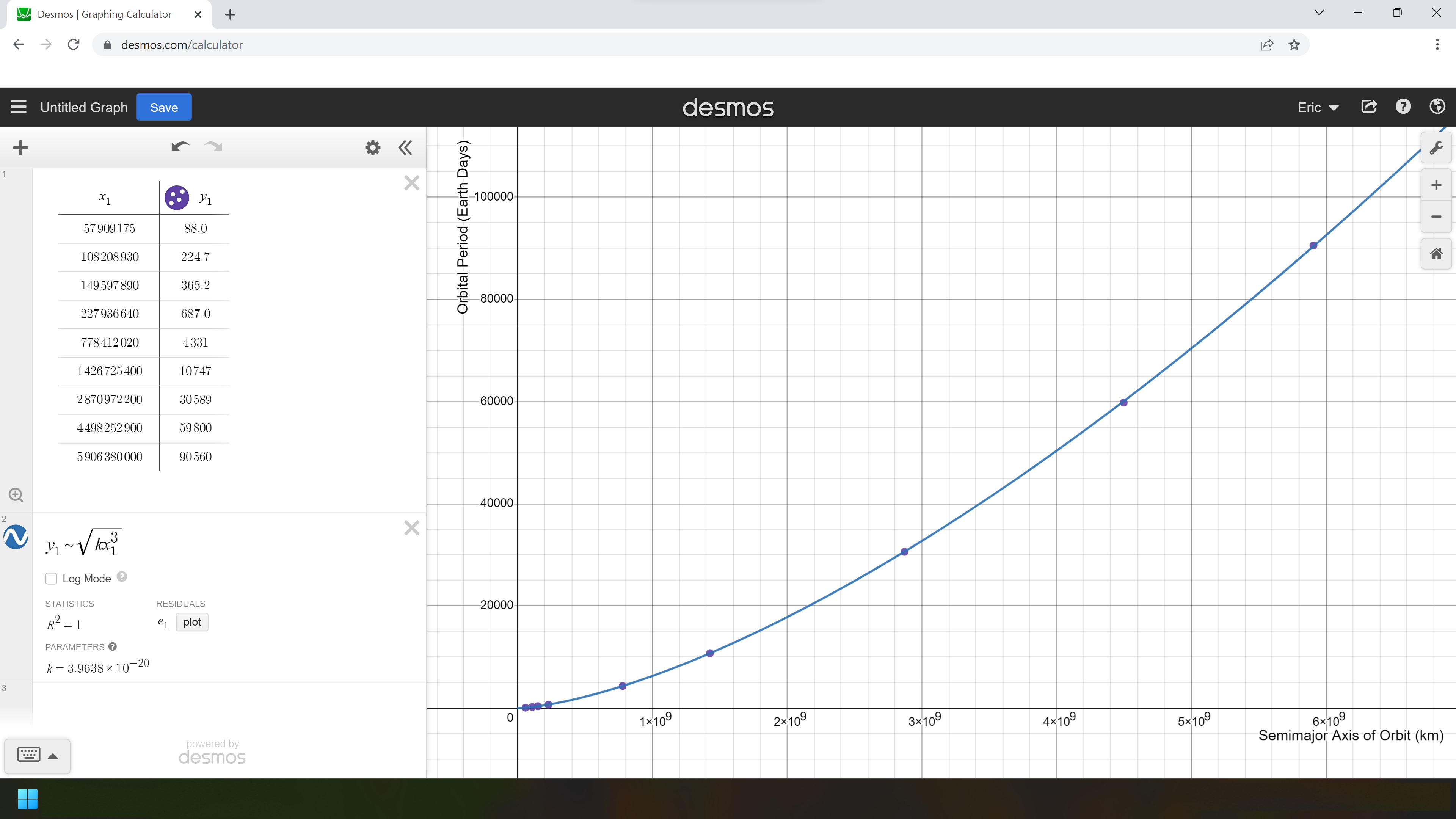Figure 2: A curve of best fit for Kepler’s third law of planetary motion, click here to access the file in Desmos.

For the previous problem, I typed “y_1~sqrtkx_1^3” into the line to generate the curve of best fit. Desmos was able to find the value for k, which in this case would be k = 3.9638 × 10^-20 day²/km³. Note that this value could have also been found by measuring the slope of the line of best fit by plotting the squares of the periods against the cubes of the distances, like so, however Desmos eliminates the need to do that, and in doing that you don’t actually get to see the true proportionality curve.

Let’s not stop there though, as there are plenty of other curves we could fit in physics. One really nasty curve that comes to mind is the type of curve you get from a damped harmonic oscillator. Suppose you set up a pendulum and then pulled it to one side and released it, allowing it to swing back and forth. You could film it and then import the video file into video analysis software, like Vernier Video Analysis or Tracker, and get a set of data looking at how the x-position of the object changes over time. The motion would be fairly periodic, so a sinusoidal fit would work nicely, but due to friction the amplitude would decrease over time, in the form of an exponential decay. A function of the form x(t) =a*e^(-bt)*sin(k(t-d))+c or x(t)=a*e^(-bt)*cos(k(t-d))+c should work perfectly for this scenario.


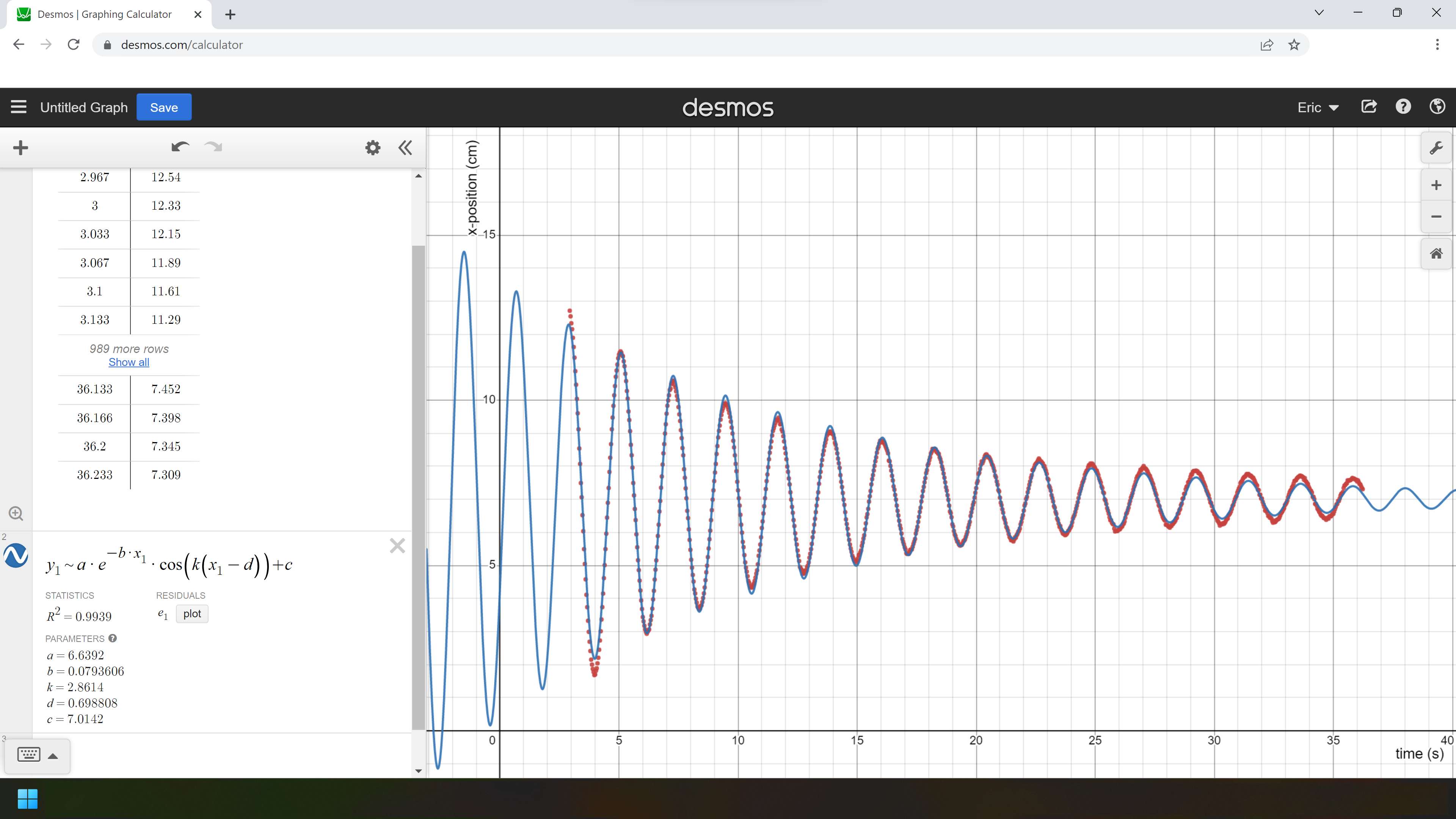Figure 3: A curve of best fit for damped harmonic motion, click here to access the file in Desmos.

Here, Desmos has done a pretty good job fitting a curve to the 1000 data points provided, and it has given us the values of the coefficients, like k = 2.8614, which tells us the frequency is f = 2π/k = 2.1905 Hz; and b = 0.0793606, which tells us the mean lifetime is 1/b = 12.6 s.

Note that I was somewhat lucky Desmos was able to find those coefficients correctly. Since the algorithm ‘walks’ the coefficients to a smaller and smaller error, it has the potential to sometimes settle upon a local minimum, rather than the global minimum. Desmos explains it better here. Sometimes, especially with more complex equations, it is necessary to eyeball the coefficients before getting Desmos to fit the curve for you. Desmos makes this process very easy, just put unknown coefficients into the equation and then click on ‘add slider: all’, and then slide the sliders around until you get a fairly close approximation. After you have a good estimate, run the curve fitting like before, but put your estimates for the coefficients next to the equation, for example, in the form of {6 < c < 8}.


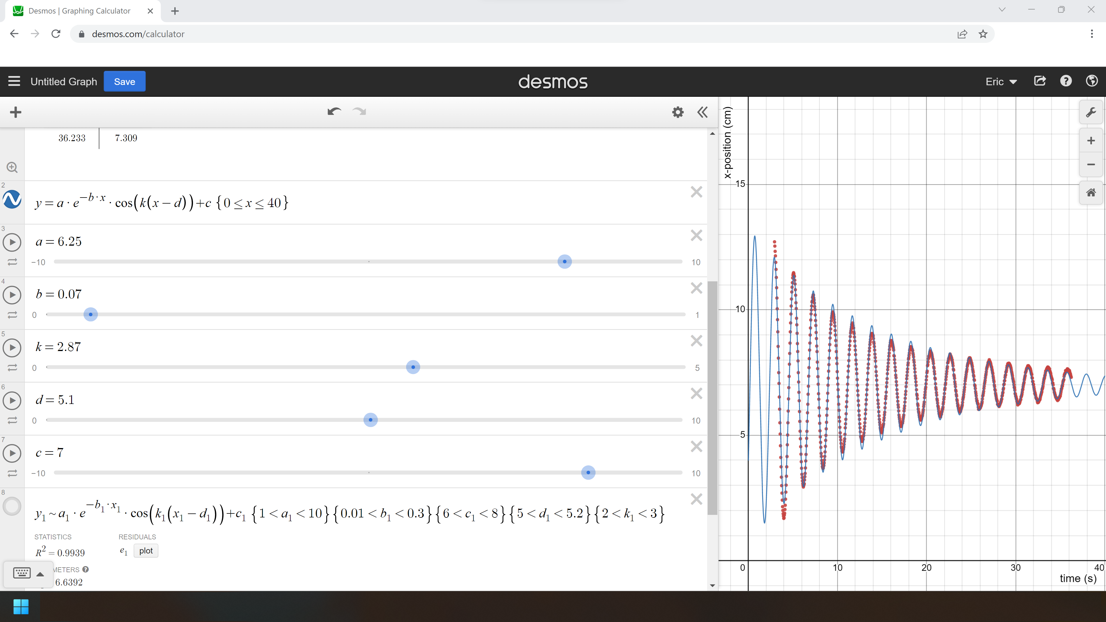Figure 4: Adding sliders allows you to easily eyeball the values for the coefficients, which is sometimes necessary to fit the curve, click here to access the file in Desmos.

In this example, notice that the first peak in the dataset happens roughly when x = 5.1. Since I was using a cosine function, that means I could use d ≐ 5.1. To enter that into Desmos, I had put {5 < d < 5.2} next to the curve fitting equation. While I was at it, I also put lower and upper bounds on the other coefficients. Notice that when Desmos originally did the curve fitting it came up with d =  0.698808, which would be the x-value of the first peak of the graph, which starts before the data points begin. When I added in the restriction on d, {5 < d < 5.2}, Desmos was able to hone in on a new value for d, this time arriving at a new local minimum for the errors, with d = 5.0905.

As an extension to fitting that curve, we could ask our students to repeat the pendulum experiment multiple times to see whether the frequency or damping coefficient changes depending on the initial displacement of the pendulum, the length of the string, or the mass of the pendulum. We could then graph those data points and fit curves to that data to find those proportionalities. This curve fitting technique be useful for other complex types of curves, like how in the second year of university in classical mechanics, you may have encountered a projectile with air resistance, which has a trajectory described by the following equation.



Also, if you have ever studied spectroscopy, you may have done labs involving complex curves that ended up looking something like this.


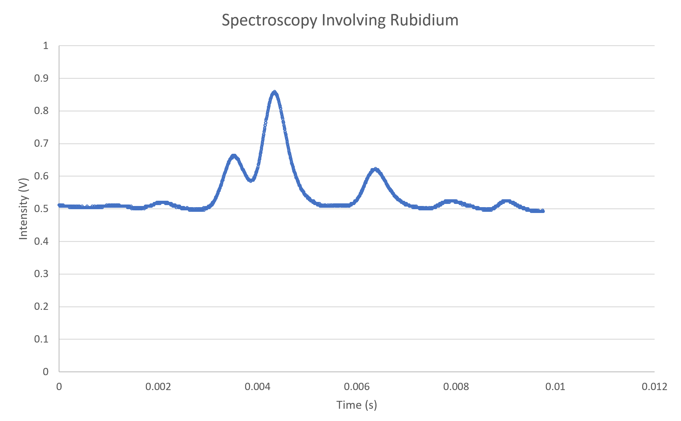Figure 5: A set of spectroscopy data I recorded in university, which I had to fit a curve to.

In addition to physics courses, this kind of curve fitting can be performed in math classes too. Grade 12 Advanced Functions (MHF4U) has a section on combining functions (unit D, specific expectation 2); the damped harmonic oscillator is an example you could cover that combines an exponential function with a sinusoidal function. Also, Desmos is great to use for fitting curves to photographs, in grade 10 math I’ll get students to fit a parabola to a photo of a parabolic arch, click here to see an example of that where you can even click and drag the points around.

I hope some of you will find this useful in your classrooms!

Tags: Math, Motion, Technology